Lecode Input XmL Structure


XML Input


Lecode is using XML input file. XML language, compared to standard ASCII, is well formatted and has a controlled structured. The XML input file has both constrains on the structure and content of the elements which are used to control the parameters of the simulation.
The XML file is at the core of the experiment design and contains all the variables and properties applicable to the simulation.
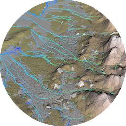
External ASCII files (formatted in CSV) are referenced inside the XML document and provide information on the basal node position, the geometry and composition of the initial layers, uplift/subsidence, rainfall and sea level...
Along side the XML input files, we developed an XML schema (XSD) file, to assist the user in setting up a particular experiment as well as to give some informations regarding the definition of the parameters used in the input files.

The XML input file is not intended to work but contains all the elements that could be declared for any particular Lecode simulations (the complete XML input file). To start with a working input file it is recommended to use one of the cookbook examples.

Header


<?xml version="1.0" encoding="UTF-8"?>
<lecode:lecodeInput xmlns:xsi="http://www.w3.org/2001/XMLSchema-instance"
  xmlns:lecode="http://subversion.assembla.com/svn/xsd/XSDlecode"
  xmlns:xi="http://www.w3.org/2001/XInclude"
  xsi:schemaLocation="http://subversion.assembla.com/svn/xsd/XSDlecode
  http://subversion.assembla.com/svn/xsd/XSDlecode/LECODE.xsd">


Mesh & TIN Declaration


The first structure which appears on the input file is related to the definition of the stratigraphic grid and flow computational grid (TIN).
Most of the elements within this structure are required.

<Strata_grid> element definitions


  <struct-Mesh-TIN>
    <Strata_grid>
      <StrataGrid>data/gbr_N.nodes</StrataGrid>
      <GridX>330</GridX>
      <GridY>330</GridY>
      <GridSpace unit="m">500</GridSpace>
      <GridXo unit="m">305250.0</GridXo>
      <GridYo unit="m">8220250.0</GridYo>
    </Strata_grid>

<StrataGrid> element: It refers to the name of the basement node file and its path. The path is from the main input file location. This ASCII file provides for each line the following information:
    ○ node IDs,
    ○ X coordinates in metres (this axis has a West to East orientation),
    ○ Y coordinates in metres (this axis has a South to West orientation), and
    ○ Z coordinates in metres.
In addition the nodes should be defined in increasing order starting from the Sout-West corner and going first along the X axis (West to East).
<GridX> element: Number of nodes along the X axis (West to East direction). It should conform with basement node file definition.
<GridY> element: Number of nodes along the Y axis (West to East direction). It should conform with basement node file definition.
<GridSpace> element: Grid spacing (in metres), defining the stratigraphic grid resolution. It should conform with basement node file definition.
<GridXo> element: South West corner X coordinate expressed in metres. It should conform with basement node file definition.
<GridYo> element: South West corner Y coordinate expressed in metres. It should conform with basement node file definition.

<TIN_refine> element definitions


    <TIN_refine>
      <HighRes unit="m">500</HighRes>
      <LowRes unit="m">1000</LowRes>
      <StepFill unit="m">0.001</StepFill>
      <FlowAcc>10</FlowAcc>
    </TIN_refine>

This elements defines the Triangular Irregular Network (TIN) . The TIN is used to compute the flow surface evolution and is automatically generated during simulation to ensure better resolution calculation in places most subject to potential flow processes.
<HighRes> element: Highest resolution for the TIN in metres. The value should be equal or higher than the stratigraphic grid spacing defined above in parameter <GridSpace>. In addition this value needs to be a multiple of the grid spacing.
<LowRes> element: Lowest resolution for the TIN in metres. The value should be equal or higher than the highest resolution defined above in parameter <HighRes >. In addition this value needs to be a multiple of the grid spacing.
<StepFill> element: Parameter used to fill all of the depressions on the stratigraphic grid topography and to remove the flat and hole areas. This is a pre-processing step used to ensure continuous flow from each grid cell. This parameter is an incremental step used during the depression filling process and is expressed in metres.
Note: in case the depression filling algorithm is not required for your simulation set the value to 0.0.
Ref: Planchon, O., and F., Darboux (2001). A fast, simple and versatile algorithm to fill the depressions of digital elevation models. Catena, 46, 159–176.

<FlowAcc> element: Flow accumulation operation performs a cumulative count of the number of pixels that naturally drain into outlets. This operation is performed several time during the simulation to adjust and adapt the TIN grid resolution depending on the areas of highest flow accumulation values. This parameter sets the minimum flow accumulation value over which the high resolution (parameter <HighRes> defined above) is used to generate the TIN resolution. For areas with flow accumulation values below this parameter the <LowRes> parameter is used.
Note: the minimum value for the flow accumulation is 1.

<Boundary> element definitions


    <Boundary>
      <North>2</North>
      <South>0</South>
      <East>0</East>
      <West>0</West>
    </Boundary>

This element specifies the model boundary types for the stratigraphic grid along all sides (North, South, East & West). For each border the following values could be set:
    ○ 0 for infinite flat boundary,
    ○ 1 to insert a wall and prevent sediment transfer and fluid loss outside the simulated domain,
    ○ 2 for extended slope.

<Restart> element definitions - This is an optional element


    <Restart>
      <RestartFolder>path/to/previous/output/Folder</RestartFolder>
      <RestartIt>40</RestartIt>
      <ProcNb>2</ProcNb>
    </Restart>
  </struct-Mesh-TIN>

It controls of the restart functionality. Model can be set to restart from a previous simulation step.
Note: This element is optional and only required to perform a simulation based on a previously simulation.
<RestartFolder> element: Name of the output folder from the previous run.
Note: it corresponds to the <OutputDirectory> parameter defined in the previous XmL input file that needs to be restarted.
<RestartIt> element: The restart iteration number is informing the code on which file ID needs to be ran from the previous simulations. Depending on how the <CheckPointing> parameters were set (if set) the software is outputting a series of checkpointing files at given time steps (See <CheckPointing> parameter for additional definition). These files are located in the runfiles directory under the folder specified in the <RestartFolder> element above and are named checkpoint.<RestartIt>.pID.h5 where <RestartIt> corresponds to a given <LayerTime> iteration number and pID to a given processor ID number
Note: You will need to ensure that the restart iteration number corresponds to the value of the simulation that you are currently defining.
Note: In case you did not set the <CheckPointing> parameter in the previous simulation the code is generating the check pointing files just for the end of your previous run which means that you should have only one <RestartIt> number and that the new simulation parameter will be equal to the <endTime> parameter of the previous one.

<ProcNb> element: Number of processors used in the last simulation. This number could be retrieved by looking at the check pointing files located in the runfiles directory under the folder specified in the <RestartFolder< element above. The number will be equal to the biggest ID of the checkpoint.<RestartIt>.pID.h5 file names plus 1.


Time Parameters


The second structure defines simulation and processes time steps.
Most of the elements within this structure are required.

<Time> element definitions

  <struct-time>
    <Time>
      <startTime unit="a">-120000</startTime>
      <endTime unit="a">-110000</endTime>
      <layerTime unit="a">1000</layerTime>
      <outputTime unit="a">2000</outputTime>
      <riverInterval unit="a">250</riverInterval>
      <rainInterval unit="a">500</rainInterval>
      <SlopeInterval unit="a">250</SlopeInterval>
      <samplingInterval unit="a">250</samplingInterval>
    </Time>

It declares general time controlling parameters.
<startTime> element: Declaration of simulation starting time in years.
Note: the start time parameter accepts both positive and negative value to represent time before present.
<endTime> element: Declaration of simulation ending time in years. Obviously, this value needs to be greater than the starting time one.
Note: the end time parameter accepts both positive and negative value to represent time before present.
<layerTime> element: Sedimentary layers are recorded through time and each layer corresponds to a specific time interval. This time interval is expressed in years.
Note: The smaller the layer time, the higher the temporal resolution of the sedimentary record will be. However it will also impact the simulation computational time so compromise needs to be made.
<outputTime> element: Time at which a new output is generated. The value should be at least equal to the layer time interval and could be set as a multiple of this parameter. In case of simulation creating large output files it is recommend to set this value to 4 or 5 times the <layerTime> one.
Note: Consider increasing the output time interval to gain save some computational time and space on your remote or local machine.
<riverInterval> element: Flow time sampling interval expressed in years. It controls how often flow walkers are released from their sources. The sources are defined in the <Sources> element and correspond to rivers or gravity currents flowing within the simulation domain.
Note: The value should be a factor of the layer time interval. In case the simulation has no sources declared set this value to a large number.
<rainInterval> element: Rain time sampling interval expressed in years. It controls how often flow walkers are released from rainfall grid. The rainfall is defined in the <RainfallGrid> element.
Note: The value should be a factor of the layer time interval. In case the simulation has no rain declared set this value to a large number.
<SlopeInterval> element: Slope diffusion time sampling interval expressed in years. It controls how often slope diffusion algorithm is used to smooth top layer newly deposited sediments.
Note: The value should be a factor of the layer time interval.
<samplingInterval> element: The sampling interval is expressed in years and controls how often sea level fluctuations, displacements are updated within the simulation.
Note: The value should be a factor of the layer time interval.

<CheckPointing> element definitions - This is an optional element

    <CheckPointing>
      <Frequency>10</Frequency>	
    </CheckPointing>
  </struct-time>

The software is not able to restart a simulation from a given time step using the output files generated. To make it possible the <CheckPointing> element needs to be set. This element enable the creation of a series of restarting files located in the runfiles directory under the folder specified in the <OutputDirectory> element. These files are named checkpoint.tID.pID.h5 where tID corresponds to a particular time iteration step and pID to a given processor ID number.
Note: This element is optional.
Note: By default the code is going to generate a checkpoint file at the end of the simulation.

<Frequency> element: Frequency at which check pointing is performed. This integer is directly linked to the layer time interval element and corresponding simulation time for a given checkpoint file is retrieved by multiplying the frequency ID number (defined as tID in explanation above) by the layer time interval and by adding the simulation starting time.


Ocean & Geodynamic Structures


Follows two optional structures which define ocean and geodynamic processes.
Most of the elements within these structures are optional.

<struct-ocean> structure definitions


<struct-ocean> defines ocean characteristics and hemipelagic processes.

  <struct-ocean>
    <SeaLevelFluctuations>
      <SeaLevelFile>data/sealevel.sl</SeaLevelFile>
    </SeaLevelFluctuations>
    <HemipelagicRates>
      <HemipelagicFile>data/hemipelagic.rates</HemipelagicFile>
    </HemipelagicRates>
    <WaterDensities>
      <enteringFluid unit="kg/m3">1.000E3</enteringFluid>
      <seaDensity unit="kg/m3">1.027E3</seaDensity>
    </WaterDensities>
  </struct-ocean>

<SeaLevelFluctuations> element: Declaration of the sea-level fluctuations.
Note: This element is optional.
<SeaLevelFile> element: Name of the sea-level fluctuations file and its associated path. The path is from the main input file location. This ASCII file provides for each line the following information:
    ○ time in years,
    ○ sea-level elevation for the considered time in metres.
In addition the defined fluctuation times should be set in increasing order starting from the oldest time.
<HemipelagicRates> element: Sedimentation rates of hemipelagic particles.
Note: This element is optional.
<HemipelagicFile> element: Name of the hemipelagic rates file and its associated path. The path is from the main input file location. This ASCII file provides for each line the following information:
    ○ contour elevation in metres relative to sea-level elevation (should be negative),
    ○ hemipelagic rates in metres per year for the considered contour line.
Note: To work correctly an hemipelagic material type is required in the <Material> element with the following Material named Hemi.
<HemipelagicRates> element: Sedimentation rates of hemipelagic particles.
Note: This element is optional.
<WaterDensities> element: Water densities declaration.
Note: This element is required.
<enteringFluid> element: Density of fresh water entering the system in kg/m3. This is the density of rivers and rain particles.
<seaDensity> element: Sea water density in kg/m3.

<struct-geodyn> structure definitions


<struct-geodyn> defines the vertical displacement rates.
Note: This structure is optional.

  <struct-geodyn>  
     <Displacement>
        <nbDispInterval>1</nbDispInterval>
        <disp>
            <startDispTime unit="a">-163000000</startDispTime>
            <endDispTime unit="a">-150000001</endDispTime>
            <dispFile>data/tectonic.disp</dispFile>
        </disp>
     </Displacement>    
  </struct-geodyn>

<Displacement> element: Definition of the vertical displacement fields within simulated spatial and temporal domain.
<nbDispInterval> element: Total number of displacement intervals that will be simulated. The displacement intervals need to be declared by increasing time and should not overlap with each others.
Note: this is not required to have the displacement start and end times continuous between each others or within the range of the sampling interval values.
<disp> element: Definition of an individual displacement field.
<startDispTime> element: Time in years at which the considered vertical displacement will start.
<endDispTime> element: Time in years at which the considered vertical displacement will end.
<dispFile> element: Name of the displacement file and its associated path. The path is from the main input file location. This ASCII file provides for each line the following information:
    ○ The node ID (which should match with one defined in the basement grid <StrataGrid>),
    ○ cumulative vertical displacement for each considered node in metres.
Attention: the file defines the cumulative displacement during the duration defined above and not a displacement rate.
Note: the nodes have been defined in increasing order starting from the Sout-West corner and going first along the X axis (West to East).


Sediments Properties


The next structure defines sediment types and characteristics as well as initial deposit layer composition.
All of the elements within these structures are required.

<struct-sediments> structure definitions

  <struct-sediments>
    <Materials>
      <NbSiliciclastics>1</NbSiliciclastics>
      <NbCarbonates>1</NbCarbonates>
      <NbOrganics>1</NbOrganics>
      <MinSlope>0.00001</MinSlope>
      <si>
        <MaterialName>slop_grav</MaterialName>
        <Diameter unit="mm">0.5</Diameter>
        <Density unit="kg/m3">2620.0</Density>
        <SlopeMarine>0.007</SlopeMarine>
        <SlopeAerial>0.00016</SlopeAerial>
      </si>
      <carb>
        <MaterialName>car_grav</MaterialName>
        <Diameter unit="mm">0.5</Diameter>
        <Density unit="kg/m3">2600.0</Density>
        <SlopeMarine>0.0141</SlopeMarine> 
        <SlopeAerial>0.002</SlopeAerial> 
      </carb>
      <org>
        <MaterialName>org_coal</MaterialName>
        <Diameter unit="mm">0.05</Diameter>
        <Density unit="kg/m3">2400.0</Density>
        <SlopeMarine>0.05</SlopeMarine> 
        <SlopeAerial>0.002</SlopeAerial> 
      </org>
    </Materials>

<Materials> element: Declaration of material classes present in the simulated domain. The definition of the material classes starts with the declaration of the siliciclastics, then the carbonates and finally the organics.
Note: The total number of materials is equal to the sum of siliciclastics, carbonates and organics. It is not required to set some materials for each type but it is required to have at least one material defined.
Note: The total number of materials is set to 10 in the default version of LECODE. If the simulation requires more grain sizes you will need to change the default value (called max_grn) within LECODE and recompile it.
Note: Each 3 types of materials needs to be organise by decreasing diameter size.

<NbSiliciclastics> element: Number of siliclastics defined for this simulation.
<NbCarbonates> element: Number of carbonates defined for this simulation.
<NbOrganics> element: Number of organics defined for this simulation.
<MinSlope> element: Minimum slope of deposited sediment taken into account for slope diffusion calculation. Below this threshold value, slope diffusion is not computed.
<si> element: Collection of siliciclastics classes.
Note: it is possible to defined two classes with the same parameters as long as they have a different name. This could be useful when looking at provenance problems.
Note: This element is optional.

<carb> element: Collection of carbonates classes.
Note: it is possible to defined two classes with the same parameters as long as they have a different name. This could be useful when looking at provenance problems.
Note: This element is optional.

<org> element: Collection of organic classes.
Note: it is possible to defined two classes with the same parameters as long as they have a different name. This could be useful when looking at provenance problems.
Note: This element is optional.

<MaterialName> element: Name of the considered sediment class.
Note: chosen names are not predefined and could be anything but should differ between each class.
Note: in case the <HemipelagicRates> element has been set, it is required for one of the sediment class to have its name set to Hemi.
<Diameter> element: Grain size diameter of the considered sediment class in millimetres.
<Density> element: Density of the considered sediment class in kg/m3.
<SlopeMarine> element: Angle of repose of the sediment siliciclastic class when deposited in marine environment. This angle is used during the diffusion process to define the stability of the newly deposited sediments.
<SlopeAerial> element: Angle of repose of the considered sediment class when deposited in above sea level. This angle is used during the diffusion process to define the stability of the newly deposited sediments.

<Init_deposit> structure definitions

    <Init_deposit>
      <LayersNb>1</LayersNb>
      <dep>
        <FileName>data/gbr_N.dep</FileName>
      </dep>
    </Init_deposit>
  </struct-sediments>

<Init_deposit> element: Declaration of initial deposit layers prior to the simulation starting time. This element allows the user to start with a predefined sediment architecture. This architecture could be composed of several layers with various thicknesses throughout the spatial area making it possible to set up initially complex geometries.
Note: if your simulation starts without any predefined sedimentary layers, you will not be able to erode the basement and it is in any case required to set up a initial layer of null thicknesses.
Note: in case of a restarted simulation the initial deposition layer declaration should not be changed from the original definition.

<LayersNb> element: Number of initial deposit layers defined.
<dep> element: Declaration of a specific sedimentary layers.
Note: the layers will be arranged one over the other based on how they were declared. Which means that the first layer will be the bottom one and the last one the top one.
Note: the layer will add up to each others starting from the basement topography defined in the element.
<FileName> element: Name of a specific deposit layer file and its path. The path is from the main input file location. This ASCII file provides for each line the following information:
    ○ node IDs,
    ○ thickness of first defined material classes on this node in metres,
    ○ thickness of second defined material classes on this node in metres,
    ○     :   :   :   :   :   :   :   :   :   :   :   :   :   :   :   :   :   :   :   :   :   :   :   :   :   :   :   :   :   :
    ○     :   :   :   :   :   :   :   :   :   :   :   :   :   :   :   :   :   :   :   :   :   :   :   :   :   :   :   :   :   :
    ○ thickness of last defined material classes on this node in metres,
    ○ sedimentary layer hardness.
Note: the hardness of a given sedimentary layer is a parameter (always positive) which defines how easy a specific layer can be eroded. A value of 1 or below means that the layer erodibility is high for this node whereas a value of 10 or above will means that the layer erodibility is low and can be seen as a cemented rock.
Note: In case a particular sediment is not present its thickness needs to be set to 0.0.
Note: the nodes have been defined in increasing order starting from the Sout-West corner and going first along the X axis (West to East)
Attention: this is a requirement to defined the various sediment class thicknesses by following the same order as the one used in the definition of the different materials. If not the initial sedimentary layers will not be set properly.


Processes definition


Follow several structures used to define the forcing processes such as rivers, rain, mass movements required to move sediments around and build up the sedimentary architectures.
Most of the elements within these structures are optional.

<StreamClass> structure definitions

  <struct-processes>
    <StreamClass>
      <NbClass>2</NbClass>
      <cl>
        <BedSlope>0.0</BedSlope>
        <WDRatio>30</WDRatio>
      </cl>
      <cl>
        <BedSlope>0.2</BedSlope>
        <WDRatio>10</WDRatio>
      </cl>
    </StreamClass>

<StreamClass> element: For each flow walker, the continuity equation is solved using a semi-empirical technique based on stream classification approach (Rosgen, 2003).
Definition of the stream parameters is dependent of the type of simulation which is set. The classification sets the width to depth ratio based on specific slope angles.
<NbClass> element: Total number of stream classes required to define river characteristics over the simulated area.
Note: the element variable should be equal or greater than 2.
<cl> element: Parameters collection for the considered stream class.
Note: the number of classes needs to be equal to the number given in the element.
<BedSlope> element: Value of the local topographic slope (dz/dx).
<WDRatio> element: Width to depth ratio for the considered slope.

<Sources> structure definitions

    <Sources>
      <totalSourcesNb>1</totalSourcesNb>
      <maxDepth unit="m">6</maxDepth>
      <sourceVal>
        <ts unit="a">-128000</ts>
        <te unit="a">10000</te>
        <recurencePerc>75.0</recurencePerc>
        <x unit="m">310709.3</x>
        <y unit="m">8325284.0</y>
        <xRange unit="m">55</xRange>
        <yRange unit="m">32</yRange>
        <streamDepth unit="m">6</streamDepth>
        <Vx unit="m/s">2.0</Vx>
        <Vy unit="m/s">2.0</Vy>
        <Q unit="m3/s">100</Q>
        <Qs unit="Mt/a">0.07</Qs>
        <sedConcentration>0 0 0 20 40 40 0</sedConcentration>
        <flowType>0</flowType>
      </sourceVal>
    </Sources>

<Sources> element: Definition of river and turbidity flows transporting sediments within the simulated domain. These flows will then erode and deposit sediments depending of their internal characteristics.
Note: This element is optional.
<totalSourcesNb> element: Total number of sources that will be activated within the domain during the entire simulated time.
<maxDepth> element: Maximum sources depth.
Note: this element controls the number of flow walkers released per sources. If <maxDepth> is lower than <streamDepth> then the source will be splitted in several flow walkers.
<sourceVal> element: Collection of parameters defining each source.
Note: the number of <sourceVal> needs to be equal to the number given in the <totalSourcesNb> element.
<ts> element: Source start time in years.
<te> element: Source end time in years.
<recurencePerc> element: Percentage of time the considered flow is active over a year.
Note: values are between 0 and 100.
<x> element: Source location along Ox within the simulated domain space (m).
Note: The simulation will crash if the location of the source is outside the simulation domain.
<y> element: Source location along Oy within the simulated domain space (m).
Note: The simulation will crash if the location of the source is outside the simulation domain.
<xRange> element: X position of the source can randomly vary from its defined location. This element defined the maximum range along along Ox (m).
Note: Set the value to 0.0 to prevent any change of position along X direction.
Note: The simulation will crash if when applying the random variation the new source position is outside the simulation domain.
<yRange> element: Y position of the source can randomly vary from its defined location. This element defined the maximum range along along Oy (m).
Note: Set the value to 0.0 to prevent any change of position along Y direction.
Note: The simulation will crash if when applying the random variation the new source position is outside the simulation domain.
<streamDepth> element: Source height (m).
Note: Depending on the value sets for the <maxDepth> element the source might be splitted in several flow walkers.
<Vx> element: Vx is the source velocity component along the X direction (m/s).
Note: negative means towards West and positive towards East.
<Vy> element: Vy is the source velocity component along the Y direction (m/s).
Note: negative means towards South and positive towards North.
<Q> element: Water flux (m3/s).
<Qs> element: Sediment discharge (Mt/year).
<sedConcentration> element: Percentage of each siliciclastic sediments defined in the source.
Note: the sum of each percentage needs to be equal to 100.
Note: this is a requirement to defined a percentage for each siliciclatic sediment defined in the <Materials> element and to follow the same order as the one used in the definition of the different siliclastic materials. If not the transported sediments will not be set properly.

<flowType> element: Definition of the source type. Two choices are available:
    ○ 0 for river stream and,
    ○ 1 for turbidity current.

<RainfallGrid> structure definitions

    <RainfallGrid>
      <rainFlowAccu>100</rainFlowAccu>
      <rainMaxFW>500</rainMaxFW>
      <rainElevation unit="m">1.5</rainElevation>
      <rainCombination>0</rainCombination>
      <rainStreamQ unit="m3/s">0.5</rainStreamQ>
      <nbRainfallInterval>1</nbRainfallInterval>
      <rain>
        <startTime unit="a">0</startTime>
        <endTime unit="a">1000000</endTime>
        <rainFile>data/ridge.rain</rainFile>
      </rain>
    </RainfallGrid>

<RainfallGrid> element: Defines rainfall parameters and regime, user specifies a series of maps files with rainfall values defined for each nodes.
Note: This element is optional.
<rainFlowAccu> element: Maximum flow accumulation value used to define the rain flow walkers places.
Note: Flow accumulation operation performs a cumulative count of the number of pixels that naturally drain into outlets.
<rainMaxFW> element: Maximum number of rain flow walkers released per flow interval time
<rainElevation> element: Flow walkers height for the rain in metres.
<rainCombination> element: Rain flow walkers combination is used to create a river based on merging of several rain flow walkers.
Note: The value is set to 0 to forbid any combination to occur and should be set to 1 otherwise.
Note: this option needs further testing.

<rainStreamQ> element: Water flux used when rain walker combination is enable to define the minimal flow rate required to transformed the merged rain walkers as a river flow walker.
Note: this option is used only if the is set to 1.
<nbRainfallInterval> element: Defines the number of rainfall series imported for the considered simulation.
<rain> element: Collection of rainfall parameters defining each rainfall series.
Note: the number of classes needs to be equal to the number given in the <nbRainfallInterval> element.
<startTime> element:Give the start time of the considered rainfall grid interval in years.
<endTime> element: Give the end time of the considered rainfall grid interval in years.
<rainFile> element: Name of the rainfall file and its associated path. The path is from the main input file location. This ASCII file provides for each line the following two informations:
    ○the node ID (which should match with one defined in the basement grid <StrataGrid>),
    ○ the averaged precipitation for each considered node in metres/year.
Note: the nodes have been defined in increasing order starting from the Sout-West corner and going first along the X axis (West to East)
Note: in case a specific node does not have any precipitation it is required to set it in the file with a 0.0 value

<MassMovement> structure definitions

    <MassMovement>
      <massFlowAccu>20</massFlowAccu>
      <massCurvature>0.0</massCurvature>
      <Aerial>
        <upSlopeArea unit="km2">2.5</upSlopeArea>
        <belowUpSlope>
          <steepnessIndex>0.31</steepnessIndex>
          <concavityIndex>0.2</concavityIndex>
        </belowUpSlope>
        <aboveUpSlope>
          <steepnessIndex>0.26</steepnessIndex>
          <concavityIndex>0.</concavityIndex>
        </aboveUpSlope>
      </Aerial>
      <Marine>
        <upSlopeArea unit="km2">2.5</upSlopeArea>
        <belowUpSlope>
          <steepnessIndex>0.31</steepnessIndex>
          <concavityIndex>0.2</concavityIndex>
        </belowUpSlope>
        <aboveUpSlope>
          <steepnessIndex>0.26</steepnessIndex>
          <concavityIndex>0.</concavityIndex>
        </aboveUpSlope>
      </Marine>
    </MassMovement>

<MassMovement> element:Parameter defining mass movements. It encompasses the following types of:
    ○ landslides,
    ○ slumps,
    ○ debris flows.
Mass movements susceptibility map is derived from empirical relationships based on surface of the upslope contributing area and slope. The relation is function of 2 additional parameters:
    ○ the steepness index and,
    ○ the concavity index.
Note: Example of such relation can be found in several literature papers such as Horton et al. (2008), Blahut et al. (2010) or Kappes et al. (2011).
Note: This element is optional.

<massFlowAccu> element: Flow accumulation threshold under which no mass movement can be initiated.
Note: Flow accumulation operation performs a cumulative count of the number of pixels that naturally drain into outlets.
<massCurvature> element: Plan curvature threshold over which no mass movements can be initiated. This threshold is expected to vary with the location and the type of mass flows, and strongly depends on the grid resolution and accuracy.
Note:in western Switzerland, Horton et al. (2013) found an optimum at -0.02 per metre. Fisher et al. (2012) considered values of -0.015 to -0.005 as more accurate for Norway.
<Aerial> element: Parameters collection for aerial mass movement.
<Marine> element: Parameters collection for marine mass movement.
<upSlopeArea> element: Surface of the upslope contributing area (km2).
Note: on a specific node, it corresponds to the product of the flow accumulation and the stratigraphic grid cell area.
<belowUpSlope> element: Parameters collection for area below the upslope contributing area.
<aboveUpSlope> element: Parameters collection for area above the upslope contributing area.
<steepnessIndex> element: Value of the steepness index.
<concavityIndex> element: Value of the concavity index.

<Carbonates-Organic> structure definitions

    <Carbonates-Organics>
      <carborgTime unit="a">250</carborgTime>
      <tempsalFile>data/temperature_salinity.csv</tempsalFile>
      <membershipfunctionNb>1</membershipfunctionNb>
      <fuzzyfunctionNb>1</fuzzyfunctionNb>
      <fuzzyruleNb>1</fuzzyruleNb>
      <membershipFunction>
        <functionName>shallow</functionName>
        <functionVariable>depth</functionVariable>
        <functionPts>3</functionPts>
        <functionSubset>
          <xypoints>0.0 0.0</xypoints>
          <xypoints>0.0 1.0</xypoints>
          <xypoints>25.0 0.0</xypoints>
        </functionSubset>
      </membershipFunction>
      <fuzzyFunction>
        <fuzzyName>slow_growth</fuzzyName>
        <fuzzyVariable>growth</fuzzyVariable> 
        <fuzzyPts>2</fuzzyPts>
        <fuzzySubset>
          <xycoords>0.0 0.0</xycoords>
          <xycoords>0.0005 1.0</xycoords>
        </fuzzySubset>
      </fuzzyFunction>
      <fuzzyRule>
        <matName>car_sand</matName>
        <fuzzyFctName>slow_growth</fuzzyFctName>
        <variableNb>1</variableNb>
        <membershipSet>
          <membershipFctName>shallow</membershipFctName>
        </membershipSet>
      </fuzzyRule> 
    </Carbonates-Organics>
  </struct-processes>

<Carbonates-Organics> element:Definition of carbonates and organics evolution within the simulated domain. The evolution is based on fuzzy logic.
Note: This element is optional.
<carborgTime> element: Carbonates and organics evolution time interval expressed in years.
Note:The value should be a factor of the layer time interval.
<tempsalFile> element: Name of the salinity and temperature file and its associated path. The path is from the main input file location. This ASCII file provides for each line the following information:
    ○ time in years,
    ○ sea temperature for the considered time in Celsius and,
    ○ sea salinity for the considered time in ppm.
Note: In addition the defined times should be set in increasing order starting from the oldest time.
<membershipfunctionNb> element: Total number of membership functions. A membership function allows to graphically represent a fuzzy set. The x-axis represents the values of a given variable, whereas the y-axis represents the degrees of membership in the [0,1] interval.
<fuzzyfunctionNb> element: Total number of fuzzy functions. In LECODE, a fuzzy function defined the evolution of carbonates / organics systems based on derived local prediction of their behaviours.
<fuzzyruleNb> element: Total number of fuzzy rules. The fuzzy rules defined the "defuzzification" process from a set of fuzzy and membership functions. It will produce for a specific carbonate / organic material a quantifiable results of its evolution for a considered set of conditions.
<membershipFunction> element: Definition of the collection of membership functions.
Note: The number of membership functions should equal the number provided in the <membershipfunctionNb> element.
Note: Simple functions are used to build membership functions. Because we are defining fuzzy concepts, using more complex functions does not add more precision.
<functionName> element: User defined membership function name.
This name in fuzzy logic is called a linguistic variable and is used to facilitate the expression of fuzzy rules.
<functionVariable> element: Default variable name to set up.
The user can choose between 14 default membership variable names listed below:
    ○ depth: water depth in metres
    ○ shore-distance: distance in metres to shoreline
    ○ river-distance: distance in metres to nearest river source
    ○ carbonate-distance: distance in metres to nearest surface exposed carbonate
    ○ organic-distance: distance in metres to nearest surface exposed organic
    ○ sedimentation-rate: sedimentation rate in metres per year
    ○ temperature: surface temperature in Celsius
    ○ salinity: degree of salinity in ppm
    ○ valley: normalise number of surrounding points uphill from the reference
point (calculated from all grid points within two grid cells):
       ○ -1 = all points downhill,
       ○ 1 = all points uphill [-1,1].
    ○ gradient: average gradient of the point (calculated from all grid points within two grid cells) negative value indicates that most surrounding points are downhill from the point.
    ○ exposed-time: time the layer has been undisturbed on the surface in years.     ○ ocean-energy: wind-induced wave and currents circulation velocity in the area in m/s. You must have the plugin <OceanPlugin> turns on.
    ○ burial: depth to which the material has been buried by subsequent deposits in metres (affects material subsurface).
    ○ age: time since the layer was deposited in years (affects material subsurface).
<functionPts> element: Number of points describing the shape of the membership function.
<functionSubset> element:Collection of points defining the membership function.
Note: The number of membership function points should equal the number provided in the <functionPts> element.
<xypoints> element: Function coordinates values.
    ○ X coordinates values refer to the values of one of 14 default variable names chosen above.
    ○ Y coordinates must be between 0 and 1.
<fuzzyFunction> element: Definition of the collection of fuzzy functions.
Note: The number of fuzzy functions should equal the number provided in the <fuzzyfunctionNb> element.
Note: The fuzzy function defined the evolution of carbonates / organics based on derived local prediction of their behaviours.
<fuzzyName> element: User defined fuzzy function name.
This name in fuzzy logic is called a linguistic variable and is used to facilitate the expression of fuzzy rules.
<fuzzyVariable> element: Default variable name to set up.
The user can choose between 14 default fuzzy function variable names listed below:
    ○ growth: function controlling carbonates or organics growth rate in metres per years.
    ○ erosion: function controlling carbonates or organics erosion rate in metres per years.
    ○ porosity: function controlling carbonates or organics porosity reduction between 0 and 1.
    ○ hardness: Function controlling carbonates or organics hardness (> 1)
<fuzzyPts> element: Collection of points defining the fuzzy function.
Note: The number of membership function points should equal the number provided in the element.
<fuzzySubset> element: Number of points describing the shape of the fuzzy logic function.
<xycoords> element: Function coordinates values.
    ○ X coordinates values refer to the values of one of 4 default variable names chosen above.
    ○ Y coordinates must be between 0 and 1.
<fuzzyRule> element: Definition of the collection of fuzzy functions.
The fuzzy rules defined the "defuzzification" process from a set of fuzzy and membership functions.
<matName> element: Name of the carbonate or organic type defined in the <Materials> element.
Note: This is one of the name (<MaterialName>) defined in the <carb> or <org> element.
<fuzzyFctName> element:Previously user defined fuzzy logic function name to be used with the considered material.
Note: This is one of the <fuzzyName> element.
<variableNb> element:Number of membership functions describing the fuzzy rule.
<membershipSet> element: Collection of membership functions used during the defuzzification process.
Note: It will produce for the chosen carbonate / organic material a quantifiable results of its evolution.
<membershipFctName> element:User defined name <functionName> used to define membership functions.
Note: The number of membership function element <membershipFctName> should equal the number provided in the <variableNb> element.


Parameters & Outputs


The next structures define additional processes parameters such as flow walkers sediment transport controlling factors and evolution of porosity and compaction in buried sedimentary layers as well as output declarations.
Most of the elements within these structures are required.

<SedimentTransportParameters> element definitions

  <struct-param>
    <SedimentTransportParameters>
      <streamMinDepth unit="m">0.05</streamMinDepth>
      <streamMaxDepth unit="m">20</streamMaxDepth>
      <streamMinWidth unit="m">1</streamMinWidth>
      <streamMaxWidth unit="m">1000</streamMaxWidth>
      <flowWalkerMinVelocity unit="m/s">0.0001</flowWalkerMinVelocity>
      <flowWalkerErosionLimit unit="m">0.25</flowWalkerErosionLimit>
      <flowWalkerDepositionLimit unit="m">0.25</flowWalkerDepositionLimit>
      <minSedimentLoad unit="t/a">0.000000000001</minSedimentLoad>
      <maxFWStepPerCell>150</maxFWStepPerCell>
    </SedimentTransportParameters>

<struct-param> element: Definition of additional processes parameters such as flow walkers sediment transport controlling factors and evoution of porosity and compaction in buried sedimentary layers.
<SedimentTransportParameters> element: Controlling factors for flow walker and sediment transport.
<streamMinDepth> element: Minimum depth for a river stream in the simulation in metres.
<streamMaxDepth> element: Maximum depth for a river stream in the simulation in metres.
<streamMinWidth> element: Minimum width for a river stream in the simulation in metres.
<streamMaxWidth> element: Maximum width for a river stream in the simulation in metres.
<flowWalkerMinVelocity> element: Minimum velocity of flow walkers (m/s) under which flow walkers are supposed to have no influence on topography.
Note: When a flow walker velocity decreases below this threshold value, all sediment load is forced to be deposited.
<flowWalkerErosionLimit> element: Maximum eroded thickness for each flow computation step in metres.
Note: This value could be set to a large number in case no limits are required regarding erosion thickness.
<flowWalkerDepositionLimit> element: Maximum deposited thickness for each flow computation step in metres.
Note: This value could be set to a large number in case no limits are required regarding deposition thickness.
<minSedimentLoad> element: Minimum sediment load threshold in tons per year under which flow walkers are supposed to have no influence on topography. Below this threshold, flow walkers are erased from the simulation.
Note:This value does not have to be modified for most of the simulations.
<maxFWStepPerCell> element: Maximum authorised number of iterations a given flow walker can remain in a stratigraphic grid cell before deposition is forced. Possible values range between 100 and 400.
Note: In flat area, flow walker velocity decreases and sediments are deposited. In some cases, the flow walker remains within a cell without really having much influence on the topography. This parameter helps to speed up the flow walker computation process by forcing deposition after a given number of time step.

<Manning> element definitions

    <Manning>
      <openchannelFlow>0.02</openchannelFlow>
      <hyperpycnalFlow>0.01</hyperpycnalFlow>
      <hypopycnalFlow>0.080</hypopycnalFlow>
    </Manning>

<Manning> element: Bottom friction coefficient for flow walker is approximated using the approach of Manning combined with a Chezy’s type form for equation. The Manning’s roughness coefficient is required for different types of flows.
<openchannelFlow> element: Coefficient for open-channel flow.
<hyperpycnalFlow> element: Coefficient for hyperpycnal flow.
<hypopycnalFlow> element: Coefficient for hypopycnal flow.

<Porosity> element definitions

    <Porosity>
      <EffPressureNb>6</EffPressureNb>
      <PorosityFile>data/porosity.por</PorosityFile>
    </Porosity>
  </struct-param>

<Porosity> elementThe porosity changes and associated compaction of burial sedimentary layers is defined as a function of grain size and lithostatic pressure expressed in MPa (also called overburden or vertical pressure).
Note: This element is optional.
<EffPressureNb> element: Number of effective pressures used to defined the porosity evolution table.
<PorosityFile> element: Name of the porosity look-up table file and its path. The path is from the main input file location.
This ASCII file provides on its first line the effective pressure values arranged by increasing order starting at 0 MPa on the surface.
Note: the lithostatic pressure gradient is usually assumed to be around 25 MPa/km.
Then follows one line for each sediment type defined in the <Materials> element. Each line contains values of porosity of the considered sediment type for the given lithostatic pressure value provided on the first line.
Note: The lines should be ordered in the same way as the declaration of the <Materials>
Note: The table forms a matrix with a number of columns equal to <EffPressureNb> and a number of lines equal to the total number of materials plus 1.

<struct-output> structure definitions

  <struct-output>
    <OutputDirectory>outSPM</OutputDirectory>
    <OutputWaterLevel>1</OutputWaterLevel>
  </struct-output>

<struct-output> element: Definition of output information.
Note: This element is required.
<OutputDirectory> element: Definition of the output directory where both simulation results and runfiles will be stored.
The directory is divided in two sub-directories:
    ○ one called "outputs" which record simulation output,
    ○ one called "runfiles" which record simulation informations
Note: the outputs sub-directory contains time-series files that can be visualised in Paraview or Visit for both the TIN grid, recorded stratigraphic mesh and flow walkers evolution.
Note: the runfiles sub-directory contains the checkpointing files required to restart a simulation.
Note: to preserve previous runs, change the output directory name otherwise it will be automatically rewritten and previous outputs will be lost.

<OutputWaterLevel> element: Sea-level fluctuations output control parameter. To save some space sea-level fluctuations outputs can be turned on and off. The value for this element can be:
    ○ 0 meaning sea-level will not need to be visualised,
    ○ 1 meaning sea-level fluctuations will be outputted (this is the default value).
Note: This element is optional.
Note: to preserve previous runs, change the output directory name otherwise it will be automatically rewritten and previous outputs will be lost.


Plugins


Definition of elements to increase LECODE modularity by interaction with other codes.
All the elements presented in this structure are optional.

<SeismicLine> element definitions

  <struct-plugin>
    <SeismicLine>
      <Xmin unit="m">1000.0</Xmin>
      <Xmax unit="m">1000.0</Xmax>
      <Ymin unit="m">30000.0</Ymin>
      <Ymax unit="m">50000.0</Ymax>
    </SeismicLine>

<SeismicLine> element: Export of a 2D pseudo seismic section. The pseudo seismic section records along the X or Y direction the sedimentary layer characteristics.
Two files are generated in the runfiles sub-directory of the output directory ( element). The first one is the seismic data itself called seismic.csv and records:
    ○ the position along the X or Y direction depending of the seismic line orientation,
    ○ the layer top elevation,
    ○ the mean grain size for the considered layer and,
    ○ the average porosity for the considered layer.
The second file represents the envelop of the seismic section and is called "envelop.csv" it records for each stratigraphic grid nodes present in the seismic line the top and bottom elevation.
Note: the export is realised at the end of the simulation.
Note: the section needs to be aligned with the mesh girding
Going beyond: These two files could then be further processed to create regularly spaced grid interpolating the seismic data values using Fatiando tools. Scripts have been developed to make this conversion and could be provided if required.

<Xmin> element: Seismic line minimum coordinate along X.
<Xmax> element: Seismic line maximum coordinate along X.
<Ymin> element: Seismic line minimum coordinate along Y.
<Ymax> element: Seismic line maximum coordinate along Y.

<RMSModel> element definitions

    <RMSModel>
      <Xmin unit="m">200300</Xmin>
      <Xmax unit="m">250300</Xmax>
      <Ymin unit="m">3928300</Ymin>
      <Ymax unit="m">4928300</Ymax>
    </RMSModel>

<RMSModel> element: Export of a geo-cellular box model defined by its X and Y minimum and maximum coordinates. The geo-cellular model records for within the defined box the sedimentary layers characteristics.
The geo-cellular file is generated in the runfiles sub-directory of the output directory (<OutputDirectory> element). The file is called "geocellular.grdecl" and records:
    ○ the coordinate of each sedimentary points within the box,
    ○ the averaged porosity and,
    ○ the proportion of each sediment types composing each sedimentary layer.
Note: the export is realised at the end of the simulation.
Note: the RMSModel plugin only works in serial.
Note: the model can be used within a reservoir model and as been tested using RMS and Temis.

<Xmin> element: Geo-cellular model minimum coordinate along X (West border).
<Xmax> element: Geo-cellular model maximum coordinate along X (East border).
<Ymin> element: Geo-cellular model minimum coordinate along Y (South border).
<Ymax> element: Geo-cellular model maximum coordinate along Y (North border).

<UnderworldPlugin> element definitions

    <UnderworldPlugin>
      <UsyncFolder>udw_lecode</UsyncFolder>
      <UsyncTime unit="a">500000</UsyncTime>
    </UnderworldPlugin>

<UnderworldPlugin> element: This plugin enable the soft coupling between Underworld geodynamic model and LECODE.
To work the plugin requires that both Underworld and Lecode have been compiled on the same machine. In Underworld specific input parameters have to be turn on to enable the coupling.
The communications between the codes are done at specific time steps and are driven by a file called 'maestro' localised in a synchronisation folder known by the 2 codes.
Lecode will provide to Underworld a VTK file containing top surface information ('topsurface.vtk').
Underworld will provide to Lecode an ASCII file containing vertical displacement fields ('uw_output.ascii').
Note: the plugin only looks at vertical displacements.
<UsyncFolder> element: Path to the synchronisation folder used by each code to read and write required coupling files.
The path is from the main input file location.
<UsyncTime> element: Time for synchronisation of LECODE and Underworld.

<OceanPlugin> element definitions

    <OceanPlugin>
      <circForcing>1</circForcing>
      <waveForcing>1</waveForcing>
      <OsyncFolder>lecode_ocean</OsyncFolder>
      <OsyncTime unit="a">500</OsyncTime>
      <morphLimit unit="m">2.5</morphLimit>
      <morphAc>500.0</morphAc>
      <nbForecast>1</nbForecast>
      <forecastClass>
        <subgroupNb>1</subgroupNb>
        <Ostart unit="a">-120000</Ostart>
        <Oend unit="a">1000</Oend>
        <subgroupProp>0.1</subgroupProp>
      </forecastClass>
    </OceanPlugin>
  </struct-plugin>

<OceanPlugin> element: Ocean plugin for waves and currents circulation. This module enable the coupling with CSIRO wave/current ocean circulation code that could be provided if requested.
The plugin allows the simulation of wind generated waves and currents circulation for various climatic scenarios.
Note: These elements need to be appropriately filled in relation to what has been set up in the ocean code input file.
<circForcing> element: Calculation of wind induced ocean currents circulation is enable if the element is set to 1 (otherwise 0).
<waveForcing> element: Calculation of wind generated wave currents is enable if the element is set to 1 (otherwise 0).
<OsyncFolder> element: Path to the synchronisation folder used by each code to read and write required coupling files.
The path is from the main input file location.
<OsyncTime> element: Time for synchronisation of LECODE and the Ocean code.
<morphLimit> element: Maximum morphological change thickness for each ocean computation step in metres.
Note: This value could be set to a large number in case no limits are required regarding morphological change.
<morphAc> element: Morphological acceleration factor. Long-term morphological evolution is achieved using hydrodynamic calculations of only a fraction of the simulated duration. This need to be calibrated based on temporal and spatial resolution of the considered simulation.
<nbForecast> element: Number of wind climate classes defined during the simulation time.
<forecastClass> element: Collection of wind hind cast parameters for each forecast class.
Note: the number of classes needs to be equal to the number given in the <nbForecast> element.
<subgroupNb> element: Number of subgroup regime defined for the considered forecast class.
Note: this needs to match with the definition provided in the ocean code input file.
<Ostart> element: Starting time of the considered forecast in year.
Note: this needs to match with the definition provided in the ocean code input file.
<Oend> element: Ending time of the considered forecast in year.
Note: this needs to match with the definition provided in the ocean code input file.
<subgroupProp> element: Proportion of time a considered wind subgroup is active over a year. The subgroup parameters such as wind velocity and direction are provided in the ocean code input file.
Note:the value for the element could not exceed 1.
Note: this needs to match with the definition provided in the ocean code input file.


Footer


</lecode:lecodeInput>